Motivations and Standard Forms

Robust LP > Motivations and standard forms | Tractable cases | Applications

The uncertainty problem
Robust optimization approach

The uncertainty problem

Data uncertainty

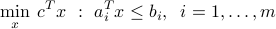
Consider the linear program in inequality form:

min_x : c^Tx ~:~ a_i^Tx le b_i , ;; i= 1,ldots,m

In practice, the data of the linear program (contained in the vectors , , and a_i , i=1,ldots,m ) are often not well-known. Solving the LP without taking into account the uncertainty in the problem's data might make the supposedly “optimal” solution very sub-optimal, or even infeasible.

Example: Uncertainty in the drug production problem.

Implementation errors

Uncertainty can originate also from implementation errors. Often, the optimal variable x^ast corresponds to a certain action or implementation process, which may be fraught with errors.

In an antenna array design problem for example, the optimal antenna weights are in reality characteristics of certain physical devices and as such cannot be implemented exactly as they are computed via the optimization model. Or, in a manufacturing process, the planned production amounts are never exactly implemented due to, say, production plant failures.

Implementation errors can result in catastrophic behavior, in the sense that when the optimal variable is impacted by such errors, the constraints might become inactive, or the cost function become much worse (higher) than thought.

Example: Antenna array design with relative implementation error.

Robust optimization approach

Main idea

In robust optimization, we assume that the data in the LP is not exactly known. We postulate that a model of uncertainty is known.

In its simplest version, we assume that the a_i 's are known to belong to a given set $mathbf{U}_i subseteq mathbf{R}^n$ . We can think of those sets as sets of confidence for the coefficients of the linear program above.

Robust counterpart

The robust counterpart to the original LP above is defined as follows.

$min_x : c^Tx ~:~ forall : a_i in mathbf{U}_i , ;; a_i^Tx le b_i , ;; i= 1,ldots,m.$

The interpretation of the above problem is that it attempts to find a solution that is feasible, independent of the particular choice of the coefficient vectors a_i within their respective sets of confidence.

The robust counterpart is always convex, independent of the shape of the sets of confidence $mathbf{U}_i$ . (Indeed, the feasible set is still the intersection of half-spaces; in contrast with the original LP, their number is can be infinite, unless $mathbf{U}_i$ are finite.)

For some classes of uncertainty sets $mathbf{U}_i$ , the robust counterpart is computationally tractable. We details three such cases, which are important in applications.

Robust half-space constraints

The feasible set of the robust counterpart is the intersection of single constraints called robust half-space constraints.

Given a subset mathbf{U} of $mathbf{R}^n$ , and b in mathbf{R} , the condition on :

$forall : a in mathbf{U} , ;; a^Tx le b ,$

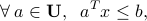
is called a robust half-space constraint. The condition is always convex, irrespective of the choice of the set mathbf{U} .

To analyze a robust half-space constraint, the main idea is to formulate it in terms of an optimization problem, as

$b ge max_{a in mathbf{U}} : a^Tx .$

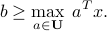
For some choices of mathbf{U} , we can solve the maximization problem explicitly.