Matrix Norms
Motivating example
RMS gain: the Frobenius norm
Peak gain: the largest singular value norm
Applications
Motivating example: effect of noise in a linear system
We saw how a matrix (say,  ) induces, via the amtrix-vector product, a linear map
  . Here,
  is an input vector and
  is the output. The mapping (that is,
  ) could represent a linear amplifier with input an audio signal and output another audio signal
  .
.
Now, assume that there is some noise in the vector : the actual input is  , where
  is an error vector. This implies that there will be noise in the output as well: the noisy output is
  , so that the error on the output due to noise is
  . How could we quantify the effect of input noise on the output noise?
One approach is to try to measure the norm of the error vector,  . Obviously, this norm depends on the noise
  , which we do not know. So we will assume that can take values in a set. We need to come up with a single number that captures in some way the different values of when spans that set. Since scaling simply scales the norm accordingly, we will restrict the vectors to have a certain norm, say
  .
.
Clearly, depending on the choice of the set, the norms we use to measure norm lengths, and how we choose to capture many numbers with one, etc, we will obtain different numbers.
RMS gain: the Frobenius norm
Let us first assume that the noise vector can take a finite set of directions, specifically the directions represented by the standard basis, . Then let us look at the average of the squared error norm:
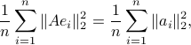
where  stands for the
  -th column of . The quantity above can be written as
  , where
is the Frobenius norm of .
The function  turns out to satisfy the basic conditions of a norm in the matrix space
  . In fact, it is the Euclidean norm of the vector of length
  formed with all the coefficients of . Further, the quantity would remain the same if we had chosen any orthonormal basis other than the standard one.
The Frobenius norm is useful to measure the RMS (root-mean-square) gain of the matrix, its average response along given mutually orthogonal directions in space. Clearly, this approach does not capture well the variance of the error, only the average effect of noise.
The computation of the Frobenius norm is very easy: it requires about flops.
>> frob_norm = norm(A,'fro');
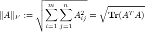
Peak gain: the largest singular value norm
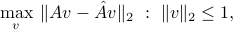
To try to capture the variance of the output noise, we may take a worst-case approach.
Let us assume that the noise vector is bounded but otherwise unknown. Specifically, all we know about is that  , where
  is the maximum amount of noise (measured in Euclidean norm). What is then the worst-case (peak) value of the norm of the output noise? This is answered by the optimization problem
The quantity

measures the peak gain of the mapping , in the sense that if the noise vector is bounded in norm by , then the output noise is bounded in norm by  . Any vector which achieves the maximum above corresponds to a direction in input space that is maximally amplified by the mapping .
The quantity  is indeed a matrix norm, called the largest singular value (LSV) norm, for reasons seen here. It is perhaps the most popular matrix norm.
The computation of the largest singular value norm of a matrix is not as easy as with the Frobenius norm. Hovewer, it can be computed with linear algebra methods seen here, in about  flops. While it is more expensive to compute than the Frobenious norm, it is also more useful because it goes beyond capturing the average response to noise.
>> lsv_norm = norm(A);
Other norms
Many other matrix norms are possible, and sometimes useful. In particular, we can generalize the notion of peak norm by using different norms to measure vector size in the input and output spaces. For example, the quantity

measures the peak gain with inputs bounded in maximum norm, and outputs measured with the  -norm.
The norms we have just introduced, the Frobenius and largest singular value norms, are the most popular ones, and are easy to compute. Many other norms are hard to compute.
Applications
Distance between matrices
Matrix norms are ways to measure the size of a matrix. This allows to quantify the difference between matrices.
Assume for example that we are trying to estimate a matrix , and came up with an estimate  . How can we measure the quality of our estimate? One way is to evaluate by how much they differ when they act on the standard basis. This leads to the Frobenius norm.
Another way is to look at the difference in the output:

when runs the whole space. Clearly, we need to scale, or limit the size, of , otherwise the difference above may be arbitrarily big. Let's look at the worst-case difference when satisfies  . We obtain
which is the largest singular value norm of the difference  .
.
Direction of maximal variance
Consider a data set described as a collection of vectors  , with
  . We can gather this data set in a single matrix
 ![A = [a_1,ldots,a_n]in mathbf{R}^{m times n}](eqs/7159446999973340990-130.png) . For simplicity, let us assume that the average vector is zero:
. For simplicity, let us assume that the average vector is zero:
Let us try to visualize the data set by projecting it on a single line passing through the origin. The line is thus defined by a vector  , which we can without loss of generality assume to be of Euclidean norm
  . The data points, when projected on the line, are turned into real numbers
  ,
,  .
.
It can be argued that a good line to project data on is one which spreads the numbers as much as possible. (If all the data points are projected to numbers that are very close, we will not see anything, as all data points will collapse to close locations.)
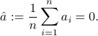
We can find a direction in space which accomplishes this, as follows. The average of the numbers is
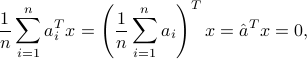
while their variance is
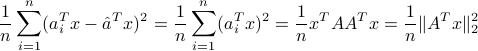
The direction of maximal variance is found by computing the LSV norm of 

(It turns out that this quantity is the same as the LSV norm of itself.)