Special Matrices
Square Matrices
Identity and diagonal matrices
Triangular matrices
Symmetric matrices
Orthogonal Matrices
Dyads
Some special square matrices
Square matrices are matrices that have the same number of rows as columns. The following are important instances of square matrices.
Identity matrix
The  identity matrix (often denoted
  , or simply
  , if context allows), has ones on its diagonal and zeros elsewhere. It is square, diagonal and symmetric. This matrix satisfies
  for every matrix
  with
with  columns, and
  for every matrix
  with rows.
>> I3 = eye(3); % the 3x3 identity matrix
>> A = eye(3,4); % a 3x4 matrix having the 3x3 identity in its first 3 columns
Diagonal matrices
Diagonal matrices are square matrices with  when
when  . A diagonal matrix can be denoted as
  , with
  the vector containing the elements on the diagonal. We can also write
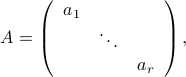
where by convention the zeros outside the diagonal are not written.
>> A = diag([1 2 3]); % a diagonal matrix with 1,2,3 on the diagonal
>> A = spdiags([1 2 3]',0,3,3); % the same matrix declared as a sparse matrix
Symmetric matrices
Symmetric matrices are square matrices that satisfy  for every pair
  . An entire section is devoted to symmetric matrices.
Triangular matrices
A square matrix  is upper triangular if when
  . Here are a few examples:
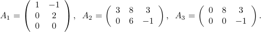
A matrix is lower triangular if its transpose is upper triangular. For example:
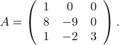
Orthogonal matrices
Orthogonal (or, unitary) matrices are square matrices, such that the columns form an orthonormal basis. If ![U = [u_1,ldots,u_n]](eqs/8584913681015734719-130.png) is an orthogonal matrix, then
is an orthogonal matrix, then
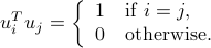
Thus,  . Similarly,
  .
.
Orthogonal matrices correspond to rotations or reflections across a direction: they preserve length and angles. Indeed, for every vector  ,
,

Thus, the underlying linear map  preserves the length (measured in Euclidean norm). This is sometimes referred to as the rotational invariance of the Euclidean norm.
In addition, angles are preserved: if  are two vectors with unit norm, then the angle
  between them satisfies
  , while the angle
  between the rotated vectors
  ,
,  satisfies
  . Since

we obtain that the angles are the same. (The converse is true: any square matrix that preserves lengths and angles is orthogonal.)
Geometrically, orthogonal matrices correspond to rotations (around a point) or reflections (around a line passing through the origin).
Examples:
 orthogonal matrix
Dyads
Dyads are a special class of matrices, also called rank-one matrices, for reasons seen later.
Definition
A matrix is a dyad if it is of the form  for some vectors
  ,
,  . The dyad acts on an input vector
  as follows:
In terms of the associated linear map, for a dyad, the output always points in the same direction  in output space (
 ), no matter what the input is. The output is thus always a simple scaled version of . The amount of scaling depends on the vector
  , via the linear function
  .
.
Example: Single-factor models of financial data.
Normalized dyads
We can always normalize the dyad, by assuming that both  are of unit (Eculidean) norm, and using a factor to capture their scale. That is, any dyad can be written in normalized form:

where  , and
, and  .
.