Matrix Products
Matrix-vector product
Matrix-matrix product
Block matrix product
Trace and scalar product
Matrix-vector product
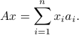
Definition
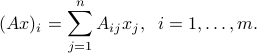
We define the matrix-vector product between a  matrix and a
  -vector
  , and denote by
  , the
, the  -vector with
  -th component
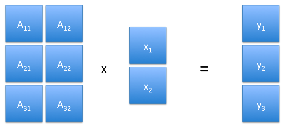 |
The picture on the left shows a symbolic example with 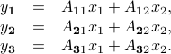
|
 and
and  . We have
  , that is:
Interpretation as linear combinations of columns
If the columns of  are given by the vectors
  ,
,  , so that
  , then can be interpreted as a linear combination of these columns, with weights given by the vector :
 |
In the above symbolic example, we have 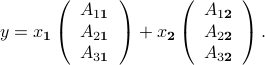
|
Example:
Interpretation as scalar products with rows
Alternatively, if the rows of are the row vectors  ,
,  :
:
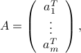
then is the vector with elements  , :
, :
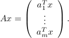
 |
In the above symbolic example, we have 
|
Example: Absorption spectrometry: using measurements at different light frequencies.
Left product
If  , then the notation
  is the row vector of size equal to the transpose of the column vector
  . That is:
Example: Return to the network example, involving a incidence matrix. We note that, by construction, the columns of sum to zero, which can be compactly written as  , or
, or  .
.
Matlab syntax
The product operator in Matlab is *. If the sizes are not consistent, Matlab will produce an error.
>> A = [1 2; 3 4; 5 6]; % 3x2 matrix
>> x = [-1; 1]; % 2x1 vector
>> y = A*x; % result is a 3x1 vector
>> z = [-1; 0; 1]; % 3x1 vector
>> y = z'*A; % result is a 1x2 (i.e., row) vector
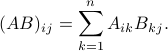
Matrix-matrix product
Definition
We can extend matrix-vector product to matrix-matrix product, as follows. If  and
and  , the notation
  denotes the
  matrix with
  element given by
Transposing a product changes the order, so that 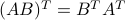 .
.
Column-wise interpretation
If the columns of  are given by the vectors
  , , so that
 ![B = [b_1 , ldots, b_n]](eqs/3204593958553039499-130.png) , then can be written as
, then can be written as

In other words, results from transforming each column of into  .
.
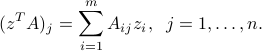
Row-wise interpretation
The matrix-matrix product can also be interpreted as an operation on the rows of . Indeed, if is given by its rows , , then is the matrix obtained by transforming each one of these rows via , into  , :
, :
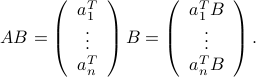
(Note that 's are indeed row vectors, according to our matrix-vector rules.)
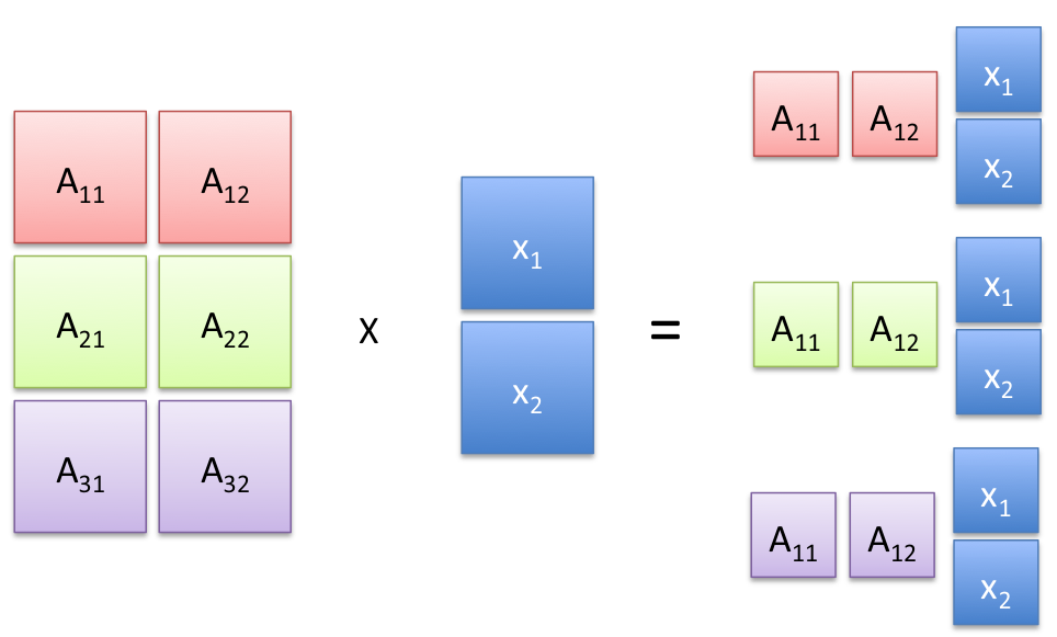
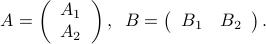
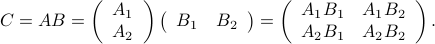
Block Matrix Products
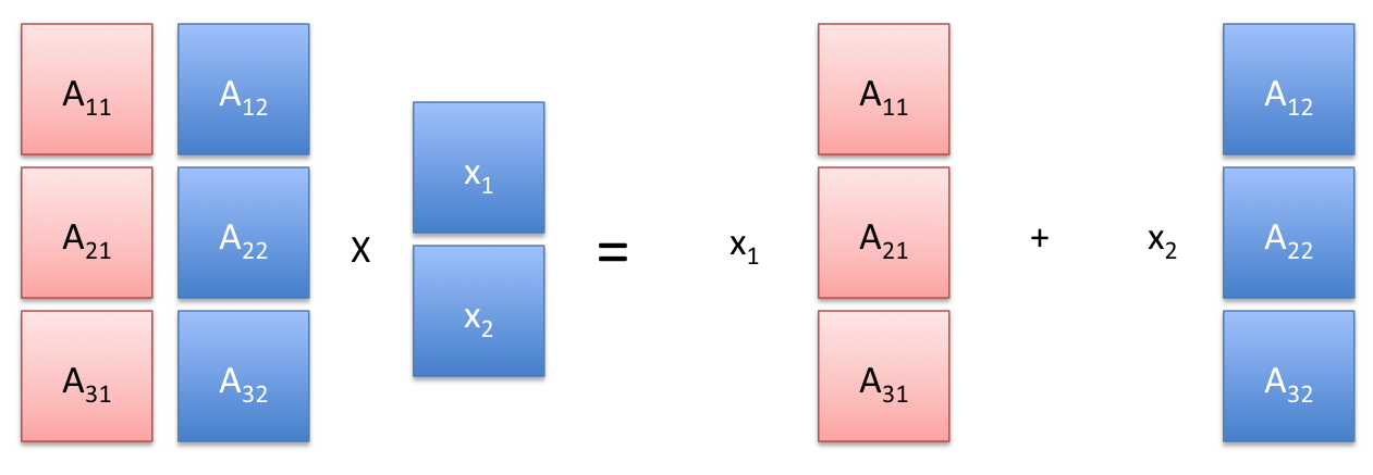
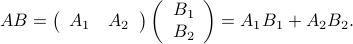
Matrix algebra generalizes to blocks, provided block sizes are consistent. To illustrate this, consider the matrix-vector product between a matrix and a -vector , where  are partitioned in blocks, as follows:
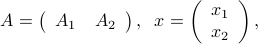
where  is
is  ,
,  ,
,  ,
,  . Then

Symbolically, it's as if we would form the ‘‘scalar’’ product between the ‘‘row vector  and the column vector
  !
!
Likewise, if a  matrix is partitioned into two blocks
  , each of size
  , , with , then
Again, symbolically we apply the same rules as for the scalar product — except that now the result is a matrix.
Example: Gram matrix.
Finally, we can consider so-called outer products. Consider the case for example when is a matrix partitioned row-wise into two blocks  , and is a matrix that is partitioned column-wise into two blocks
  :
:
Then the product  can be expressed in terms of the blocks, as follows:
Trace, scalar product
Trace
The trace of a square  matrix , denoted by
  , is the sum of its diagonal elements:
 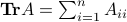 .
.
Some important properties:
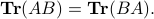
Trace of transpose: The trace of a square matrix is equal to that of its transpose.
Commutativity under trace: for any two matrices
and  , we have
>> A = [1 2 3; 4 5 6; 7 8 9]; % 3x3 matrix
>> tr = trace(A); % trace of A
Scalar product between matrices
We can define the scalar product between two matrices  via
via
The above definition is symmetric: we have

Our notation is consistent with the definition of the scalar product between two vectors, where we simply view a vector in  as a matrix in
  . We can interpret the matrix scalar product as the vector scalar product between two long vectors of length
  each, obtained by stacking all the columns of on top of each other.
>> A = [1 2; 3 4; 5 6]; % 3x2 matrix
>> B = randn(3,2); % random 3x2 matrix
>> scal_prod = trace(A'*B); % scalar product between A and B
>> scal_prod = A(:)'*B(:); % this is the same as the scalar product between the
                            % vectorized forms of A, B