Senate Voting: Principal Component Analysis
Direction of maximal variance
PCA of Senate voting matrix
Low rank approximation
Direction of maximal variance
Motivation
We have seen here how we can choose a direction in bill space, and then project the Senate voting data matrix on that direction, in order to visualize the data along a single line. Clearly, depending on how we choose the line, we will get very different pictures. Some show large variation in the data, others seems to offer a narrower range, even if we take care to normalize the directions.
What could be a good criterion to choose the direction we project the data on?
It can be argued that a direction that results in large variations of projected data is preferable to a one with small variations. A direction with high variation ‘‘explains’’ the data better, in the sense that it allows to distinguish between data points better. One criteria that we can use to quantify the variation in a collection of real numbers is the sample variance, which is the sum of the squares of the differences between the numbers and their average.
Solving the maximal variance problem
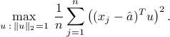
Let us find a direction which maximizes the empirical variance. We seek a (normalized) direction  such that the empirical variance of the projected values
  ,
,  , is large. If
  is the vector of averages of the
  's, the n the avarage of the projected values is
  . Thus, the direction of maximal variance is one that solves the optimization problem
The above problem can be formulated as
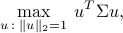
where
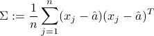
is the  sample covariance matrix of the data. The interpretation of the coefficient
  is that it provides the covariance between the votes of Senator
  and those of Senator
  .
.
We have see the above problem before, under the name of the Rayleigh quotient of a symmetric matrix. Solving the problem entails simply finding an eigenvector of the covariance matrix  that corresponds to the largest eigenvalue.
 |
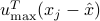
This image shows the scores assigned to each Senator along the direction of maximal variance, Note that the largest absolute score (about 18) obtained in this plot is about three times bigger than that observed on the previous one. This is consistent with the fact that the current direction has maximal variance. |
 ,
,  , with
  a normalized eigenvector corresponding to the largest eigenvalue of the covariance matrix
 Principal component analysis
Main idea
The main idea behind principal components analysis is to first find a direction that corresponds to maximal variance between the data points. The data is then projected on the hyperplane orthogonal of that direction. We obtain a new data set, and find a new direction of maximal variance. We may stop the process when we have collected enough directions (say, three if we want to visualize the data in 3D).
Mathematically, the process amounts to finding the eigenvalue decomposition of a positive semi-definite matrix: the covariance matrix of the data points. The directions of large variance correspond to the eigenvectors with the largest eigenvalues of that matrix. The projection to use to obtain, say, a two-dimensional view with the largest variance, is of the form  , where
 ![P= [u_1,u_2]^T](eqs/6280320031663741366-130.png) is a matrix that contains the eigenvectors corresponding the the first two eigenvalues.
is a matrix that contains the eigenvectors corresponding the the first two eigenvalues.
Low rank approximations
In some cases, we are not specifically interested in visualizing the data, but simply to approximate the data matrix with a ‘‘simpler’’ one.
Assume we are given a (sample) covariance matix of the data, . Let us find the eigenvalue decomposition of :
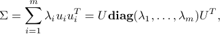
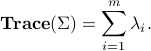
where  is an orthogonal matrix. Note that the trace of that matrix has an interpretation as the total variance in the data, which is the sum of all the variances of the votes of each Senator:
Now let us plot the values of  's in decreasing order.
 |
This image shows the eigenvalues of the |
Clearly, the eigenvalues decrease very fast. One is tempted to say that ‘‘most of the information’’ is contained in the first eigenvalue. To make this argument more rigorous, we can simply look at the ratio
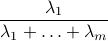
which is the ratio of the total variance in the data (as approximated by  to that of the whole matrix .
In the Senate voting case, this ratio is of the order of  . It turns out that this is true of most voting patterns in democracies across history: the first eigenvalue ‘‘explains most of the variance’’.