Senate Voting: Projecting Data

Senate Voting > Data | Projections | PCA | Sparse PCA

Projection on a line
Projection on a plane

Projecting on a line

To simplify, let us first consider the simple problem of representing the high-dimensional data set on a simple line, using the method described here.

Scoring Senators

Specifically we would like to assign a single number, or ‘‘score’’, to each column of the matrix. We choose a direction $u in mathbf{R}^m$ , and a scalar v in mathbf{R} . This corresponds to the affine ‘‘scoring’’ function $f : mathbf{R}^m rightarrow mathbf{R}$ , which, to a generic column $x in mathbf{R}^m$ of the data matrix, assigns the value

We thus obtain a vector of values $f in mathbf{R}^n$ , with f_j = u^Tx_j+v , j=1,ldots,n . It is often useful to center these values around zero. This can be done by choosing such that

$0 = sum_{j=1}^n ( u^Tx_j+v ) = u^Tleft( sum_{j=1}^n x_j right) + n cdot v,$

that is: $v = -u^That{x}$ , where

$hat{x} := frac{1}{n} sum_{j=1}^n x_j in mathbf{R}^m$

is the vector of sample averages across the columns of the matrix (that is, data points). The vector hat{x} can be interpreted as the ‘‘average response’’ across experiments.

The values of our scoring function can now be expressed as

$f(x) = u^T(x-hat{x}).$

In order to be able to compare the relative merits of different directions, we can assume, without loss of generality, that the vector is normalized (so that |u|_2 = 1 ).

Centering data

It is convenient to work with the ‘‘centered’’ data matrix, which is

$X_{rm cent} = left( begin{array}{ccc} x_1 -hat{x} & ldots x_n - hat{x} end{array}right) = X - hat{x}mathbf{1}_n^T,$

where $mathbf{1}_n$ is the vector of ones in $mathbf{R}^n$ .

In matlab, we can compute the centered data matrix as follows.

Matlab syntax
>> xhat = mean(X,2);
>> [m,n] = size(X);
>> Xcent = X-xhat*ones(1,n);

We can compute the (row) vector scores using the simple matrix-vector product:

$f = u^TX_{rm cent} in mathbf{R}^{1 times m}.$

We can check that the average of the above row vector is zero:

$fmathbf{1}_n = u^TX_{rm cent}mathbf{1}_n = u^T(X - hat{x}mathbf{1}_n^T) mathbf{1}_n = u^T(Xmathbf{1}_n - n cdot hat{x}) = 0.$

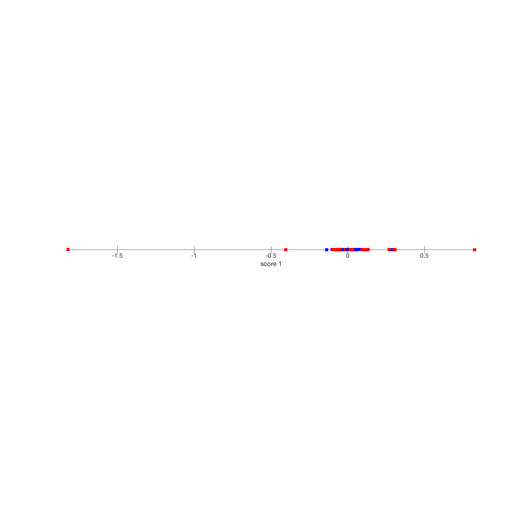
Example: visualizing along random direction

Scores obtained with random direction: This image shows the values of the projections of the Senator's votes $x_j-hat{x}$ (that is, with average across Senators removed) on a (normalized) ‘‘random bill’’ direction. This projection shows no particular obvious structure. Note that the range of the data is much less than obtained with the average bill shown above.

Projection on a plane

We can also try to project the data on a plane, which involves assigning two scores to each data point.

Scoring map

This corresponds to the affine ‘‘scoring’’ map $f : mathbf{R}^m rightarrow mathbf{R}$ , which, to a generic column $x in mathbf{R}^m$ of the data matrix, assigns the two-dimensional value

$f(x) = left( begin{array}{c} u_1^Tx + v_1 u_2^Tx+v_2 end{array}right) = U^Tx + v,$

where $u_1,u_2 mathbf{R}^m$ are two vectors, and v_1,v_2 two scalars, while $U = [u_1,u_2]in mathbf{R}^{m times 2}$ , $v in mathbf{R}^2$ .

The affine map allows to generate two-dimensional data points (instead of -dimensional) f_j = U^Tx_j+v , j=1,ldots,n . As before, we can require that the f_j 's be centered:

$0 = sum_{j=1}^n f_j = sum_{j=1}^n (U^Tx_j+v) ,$

by choosing the vector to be such that $v = -U^That{x}$ , where $hat{x} in mathbf{R}^m$ is the ‘‘average response’’ defined above. Our (centered) scoring map takes the form

$f(x) = U^T(x-hat{x}).$

We can encapsulate the scores in the 2 times n matrix F=[f_1,ldots,f_n] . The latter can be expressed as the matrix-matrix product

$F = U^TX_{rm cent} = left( begin{array}{c} u_1^TX_{rm cent} u_2^TX_{rm cent} end{array}right),$

with $X_{rm cent}$ the centered data matrix defined above.

Clearly, depending on which plan we choose to project on, we get a very different pictures. Some planes seem to be more ‘‘informative’’ than others. We return to this issue here.

Two-dimensional projection of the Senate voting matrix: This particular projection does not seem to be very informative. Notice in particular, the scale of the vertical axis. The data is all but crushed to a line, and even on the horizontal axis, the data does not show much variation.

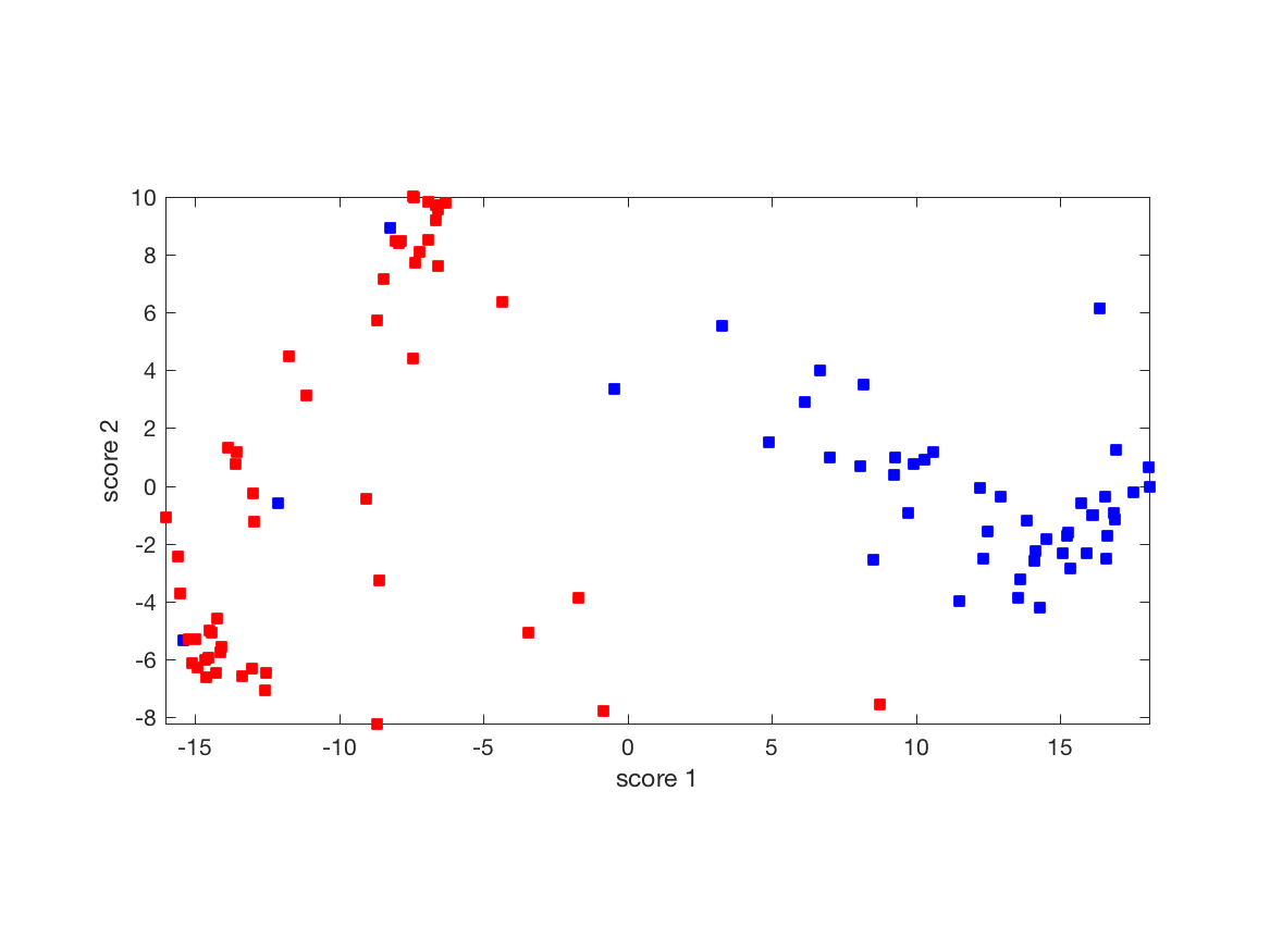Two-dimensional projection of the Senate voting matrix: This particular projection seems to allow to cluster the Senators along party line, and is therefore more informative. We explain how choose such a direction here.