Sparse PCA

Motivation

Recall that the direction of maximal variance is one vector \(\boldsymbol{u}\in\mathbb{R}^{m}\) that solves the optimization problem

\[ \max{}_{\boldsymbol{u}:\|\boldsymbol{u}\|_{2}=1}\frac{1}{n}\sum{}_{j=1}^{n}((\boldsymbol{x}_{j}-\hat{a})^{T}\boldsymbol{u})^{2} \Leftrightarrow max_{\boldsymbol{u}:\|\boldsymbol{u}\|_{2}=1}\boldsymbol{u}^{T}\boldsymbol{\Sigma}\boldsymbol{u} ,\text{where }\boldsymbol{\Sigma}=\frac{1}{n}\sum{}_{j=1}^{n}(\boldsymbol{x}_{j}-\hat{a})^{T}(\boldsymbol{x}_{j}-\hat{a}) \]

Here \(\hat{a}=\frac{1}{n}\sum_{j=1}^{n}x_{j}\) is the estimated center. We obtain a new data set by combining the variables according to the directions determined by \(\boldsymbol{u}\). The resulting dataset would have the same dimension as the original dataset, but each dimension has a different meaning (since they are linear projected images of the original variables).

As explained, the main idea behind principal components analysis is to find those directions that corresponds to maximal variances between the data points. The data is then projected on the hyperplane spanned by these principal components. We may stop the process when we have collected enough directions in the sense that the new directions explain the majority of the variance. That is, we can pick those directions corresponding to the highest scores.

We may also wonder if \(\boldsymbol{u}\) can have only a few non-zero coordinates. For example, if the optimal direction \(\boldsymbol{u}\) is \((0.01,0.02,200,100)\in\mathbb{R}^{4}\), then it is clear that the 3rd and 4th bills are characterizing most features and we may simply want to drop the 1st and 2nd bills. That is, we want to adjust the optimal direction vector as \((0,0,200,100)\in\mathbb{R}^{4}\). This adjustment accounts for sparsity. In the setting of PCA analysis, each principal component is linear combinations of all input variables. Sparse PCA allows us to find principal components as linear combinations that contain just a few input variables (hence it looks “sparse” in the input space). This feature would enhance the interpretability of the resulting dataset and perform dimension reduction in the input space. Reducing the number of input variables would assist us in the senate voting dataset, since there are more bills (input variables) than senators (samples).

This image shows the scores assigned to each Senator along the direction of maximal variance, \(u_{\rm max}^T(x_j-\hat{x})\), \(j=1,\ldots,n\), with \(u_{\rm max}\) corresponding to the PCA optimization problem, Republican Senators tend to score positively, while we find many Democrats on the negative score. Hence the direction could be interpreted as revealing the party affiliation. We are going to compare this result of PCA to sparse PCA results below.

Sparse maximal variance problem

Main idea

A mathematical generalization of the PCA can be obtained by modifying the PCA optimization problem above. We attempt to find direction of maximal variance is one vector \(\boldsymbol{u}\in\mathbb{R}^{m}\) that solves the optimization problem

\[ \max{}_{\boldsymbol{u}:\|\boldsymbol{u}\|_{2}=1,\|\boldsymbol{u}\|_{0}\leq k}\frac{1}{n}\sum{}_{j=1}^{n}((\boldsymbol{x}_{j}-\hat{a})^{T}\boldsymbol{u})^{2} \Leftrightarrow max_{\boldsymbol{u}:\|\boldsymbol{u}\|_{2}=1,\|\boldsymbol{u}\|_{0}\leq k}\boldsymbol{u}^{T}\boldsymbol{\Sigma}\boldsymbol{u} , \]

where \(\boldsymbol{\Sigma}=\frac{1}{n}\sum{}_{j=1}^{n}(\boldsymbol{x}_{j}-\hat{a})^{T}(\boldsymbol{x}_{j}-\hat{a})\). The difference is that we put one more constraint \(\|\boldsymbol{u}\|_{0}\leq k\), where \(\|\boldsymbol{u}\|_{0}\) is the number of non-zero coordinates in the vector \(\boldsymbol{u}\). For instance, \(\left\Vert (0.01,0.02,200,100)\right\Vert _{0}=4\) but \(\left\Vert (0,0,200,100)\right\Vert _{0}=2\). Here, \(k\) is a pre-determined hyper-parameter that describes the sparsity of the input space we want.This constraint of \(\|\boldsymbol{u}\|_{0}\leq k\) makes the optimization problem non-convex, and without analytically closed solution. But we still have numerical solution and the sparse properties as we explained. But \(\|\boldsymbol{u}\|_{0}\) makes the optimization problem not convex, and is difficult to solve. Instead, we practice an \(L_{1}\) regularization relaxation alternative

\[ \max{}_{\boldsymbol{u}:\|\boldsymbol{u}\|_{2}=1}\frac{1}{n}\sum{}_{j=1}^{n}((\boldsymbol{x}_{j}-\hat{a})^{T}\boldsymbol{u})^{2}+\lambda\|\boldsymbol{u}\|_{1} \Leftrightarrow max_{\boldsymbol{u}:\|\boldsymbol{u}\|_{2}=1}\boldsymbol{u}^{T}\boldsymbol{\Sigma}\boldsymbol{u}+\lambda\|\boldsymbol{u}\|_{1} . \]

This optimization problem is convex and can be solved numerically, this is the so-called sparse PCA (SPCA) method. The \(\lambda\) parameter is a pre-determined hyper-parameter we introduced as a penalty parameter, which can be tuned, as we shall see below.

Ananlysis on the senate dataset

We can apply the SPCA method onto the senate voting dataset, with \(\lambda=0\) (i.e. PCA) and increase \(\lambda=1,10,1000\). In each setting, we also record the number of non-zero coordinates of \(\boldsymbol{u}_{max}\), which is a solution to the SPCA optimization problem above. Since each coordinate of \(\boldsymbol{u}_{max}\) represents the voting outcome of one bill, we call the number of non-zero coordinates of \(\boldsymbol{u}_{max}\) as the number of active variables. From the results below, we did not observe much changes of the separation of part lines given by the principle components. As \(\lambda\) increases to 1000, there are only 7 active variables left. The corresponding 7 bills are important to separate party-line of senators, these bills are:

• 8 Energy Issues_LIHEAP Funding Amendment 3808

• 16 Abortion Issues Unintended Pregnancy Amendment 3489

• 34 Budget, Spending and Taxes Hurricane Victims Tax Benefit Amendment 3706

• 36 Budget, Spending and Taxes Native American Funding Amendment 3498

• 47 Energy Issues Reduction in Dependence on Foreign Oil 3553

• 59 Military Issues Habeas Review Amendment_3908

• 81 Business and Consumers Targeted Case Management Amendment 3664

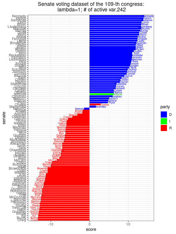This image shows the scores assigned to each Senator along the direction of maximal variance, \(u_{\rm max}^T(x_j-\hat{x})\), \(j=1,\ldots,n\), where the \(u_{\rm max}\) corresponds to the sparse PCA optimization problem with \(\lambda=1\), There are 242 non-zero coefficients, meaning that we only need 242 different bills to get this score revealing the party affiliation to this extent. This is almost identical to the result obtained from PCA.

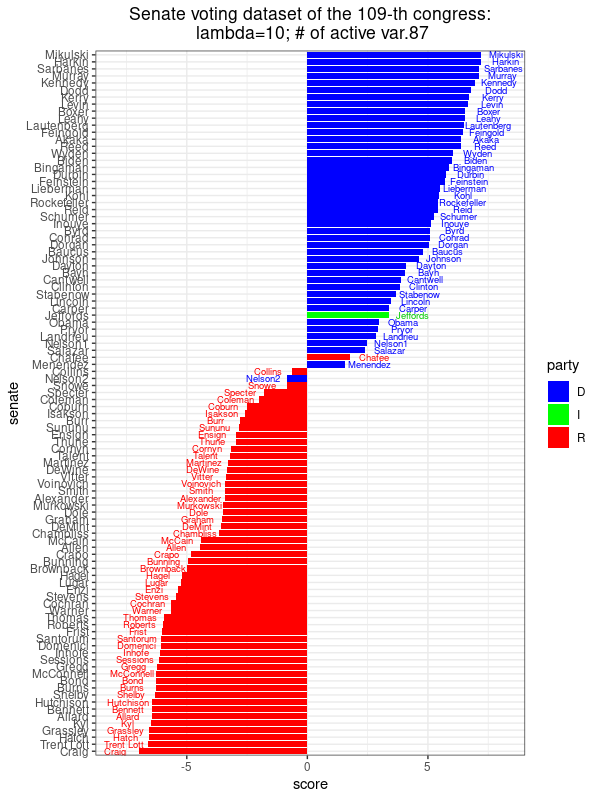This image shows the scores assigned to each Senator along the direction of maximal variance, \(u_{\rm max}^T(x_j-\hat{x})\), \(j=1,\ldots,n\), where the \(u_{\rm max}\) corresponds to the sparse PCA optimization problem with \(\lambda=10\), There are 87 non-zero coefficients, meaning that we only need 87 different bills to get this score revealing the party affiliation to this extent. Compared to PCA, there is one more mis-classified senator.

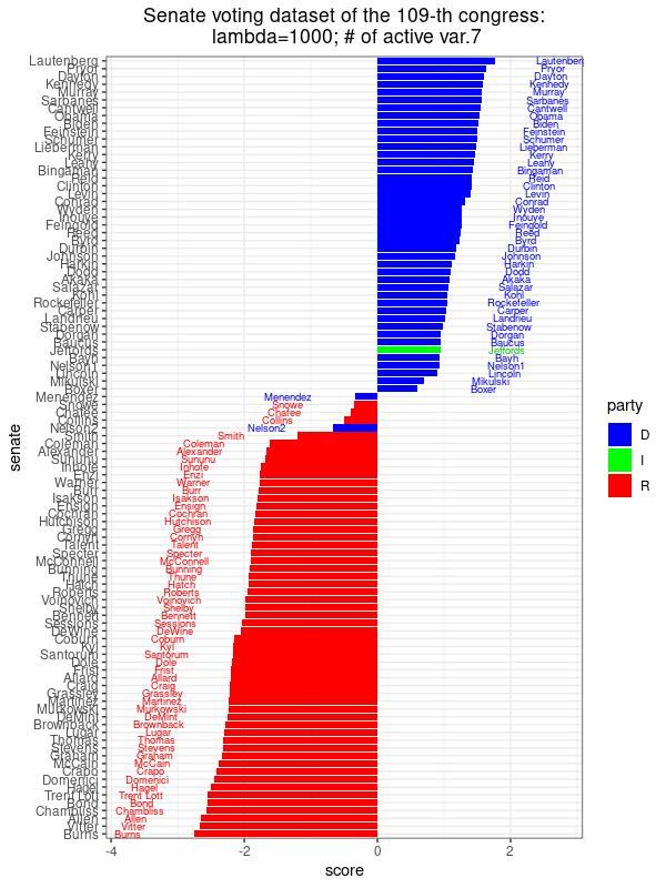This image shows the scores assigned to each Senator along the direction of maximal variance, \(u_{\rm max}^T(x_j-\hat{x})\), \(j=1,\ldots,n\), where the \(u_{\rm max}\) corresponds to the sparse PCA optimization problem with \(\lambda=1000\), There are 8 non-zero coefficients, meaning that we only need 8 different bills to get this score revealing the party affiliation to this extent, which is not much different from PCA using all 542 votes as in PCA.