Low-rank approximation of a matrix

Low-rank approximations
Link with PCA

Low-rank approximations

We consider a matrix $A in mathbf{R}^{m times n}$ , with SVD given as in the SVD theorem:

where the singular values are ordered in decreasing order, 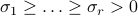sigma_1 ge ldots ge sigma_r>0

. In many applications it can be useful to approximate

with a low-rank matrix.

Example: Assume that

contains the log-returns of

assets over

time periods, so that each column of

is a time-series for a particular asset. Approximating

by a rank-one matrix of the form pq^T

, with $p in mathbf{R}^m$ and $q in mathbf{R}^n$ amounts to model the assets’ movements as all following the same pattern given by the time-profile

, each asset's movements being scaled by the components in

. Indeed, the (t,i)

component of

, which is the log-return of asset

at time

, then expresses as p(t)q(i)

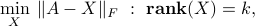
where

(

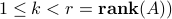is given. In the above, we measure the error in the approximation using the Frobenius norm; using the largest singular value norm leads to the same set of solutions

Theorem: Low-rank approximation

A best -rank approximation $hat{A}_k$ is given by zeroing out the r-k trailing singular values of , that is

$hat{A}_k = U hat{ {S}}_k V^T, ;; hat{ {S}}_k = mbox{bf diag}(sigma_1,ldots,sigma_k,0,ldots,0).$

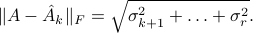
The minimal error is given by the Euclidean norm of the singular values that have been zeroed out in the process:

$|A-hat{A}_k|_F = sqrt{sigma_{k+1}^2 + ldots + sigma_r^2} .$

Sketch of proof: The proof rests on the fact that the Frobenius norm, is invariant by rotation of the input and output spaces, that is, |U^TBV|_F = |B|_F

for any matrix

, and orthogonal matrices U,V

of appropriate sizes. Since the rank is also invariant, we can reduce the problem to the case when A = tilde{S}

Link with Principal Component Analysis

Principal Component Analysis operates on the covariance matrix of the data, which is proportional to AA^T

, and sets the principal directions to be the eigenvectors of that (symmetric) matrix. As noted here, the eigenvectors of AA^T

are simply the left singular vectors of

. Hence, both methods, the above approximation method and PCA, rely on the same tool, the SVD. The latter is a more complete approach as it also provides the eigenvectors of A^TA

, which can be useful if we want to analyze the data in terms of rows instead of columns.

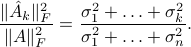
In particular, we can express the explained variance directly in terms of the singular values. In the context of visualization, the explained variance is simply the ratio to the total amount of variance in the projected data, to that in the original. More generally, when we are approximating a data matrix by a low-rank matrix, the explained variance compares the variance in the approximation to that in the original data. We can also interpret it geometrically, as the ratio of squared norm of the approximation matrix to that of the original matrix:

$frac{|hat{A}_k|_F^2}{|A|_F^2} = frac{sigma_1^2 + ldots + sigma_k^2}{sigma_1^2 + ldots + sigma_n^2} .$