Solving Linear Equations via SVD
Solution set of a linear equation
Pseudo-inverse
Sensitivity analysis and condition number
Solution set
Consider a linear equation

where  and
and  are given. We can completely describe the set of solutions via SVD, as follows. Let us assume that
  admits an SVD given here. With
  , pre-multiply the linear equation by the inverse of
  ,
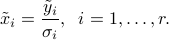
,  ; then we express the equation in terms of the rotated vector
  . This leads to

where  is the ‘‘rotated’’ right-hand side of the equation. Due to the simple form of
  , the above writes

Two cases can occur.
If the last
 components of
  are not zero, then the above system is infeasible, and the solution set is empty. This occurs when
  is not in the range of .
If
is in the range of , then the last set of conditions in the above system hold, and we can solve for  with the first set of conditions:
The last  components of are free. This corresponds to elements in the nullspace of . If is full column rank (its nullspace is reduced to
  ), then there is a unique solution.
Pseudo-inverse
Definition
The solution set is conveniently described in terms of the pseudo-inverse of , denoted by  , and defined via the SVD of :

as one with same SVD, with non-zero singular values inverted, and the matrix  transposed:

The pseudo-inverse of a matrix is always well-defined, and that it has the same size as the transpose  . When the matrix is invertible (it is square and full column or row rank:
  ), then it reduces to the inverse.
Example: pseudo-inverse of a  matrix.
>> Adagger = pinv(A);
Link with solution set
From the above development, we see that the solution set can be written as
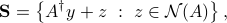
where  is the nullspace of . Both and a basis for the nullspace can be computed via the SVD.
Case when is full rank
If is full column rank, the pseudo-inverse can be written as
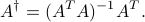
In that case, is a left-inverse of , since  .
.
If is full row-rank, then the pseudo-inverse can be written as
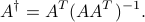
In that case, is a right-inverse of , since  .
.
Sensitivity analysis and condition number
Sensitivity analysis refers to the process of quantifying the impact of changes in the linear equations’ coefficients (the matrix and vector ), on the solution. To simplify, let us assume that is square and invertible, and analyze the effects of errors in only. The condition number of the matrix quantifies this.
We start from the linear equation above, which has the unique solution  . Now assume that is changed into
  , where
  is a vector that contains the changes in . Then let us denote by
  the new solution, which is
  . From the equations

and via the definition of the largest singular value norm, we obtain:

Combining the two inequalities we obtain:
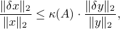
where  is the condition number of , defined as
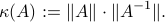
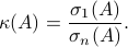
We can express the condition number as the ratio between the largest and smallest singular values of :
The condition number gives a bound on the ratio between the relative error in the left-hand side to that of the solution. We can also analyze the effect of errors in the matrix itself on the solution. The condition number turns out to play a crucial role there as well.