The SVD theorem
The SVD theorem
Geometry
Link with the spectral theorem
The SVD theorem
Basic idea
Recall from here that any matrix  with rank one can be written as

where  ,
,  , and
, and  .
.
It turns out that a similar result holds for matrices of arbitrary rank  . That is, we can express any matrix with rank one as sum of rank-one matrices
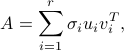
where  are mutually orthogonal,
  are also mutually orthogonal, and the
  's are positive numbers called the singular values of
  . In the above, turns out to be the rank of .
Theorem statement
The following important result applies to any matrix , and allows to understand the structure of the mapping  .
.
An arbitrary matrix admits a decomposition of the form
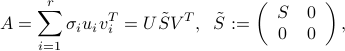
where  ,
,  are both orthogonal matrices, and the matrix
  is diagonal:
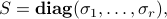
where the positive numbers 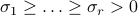 are unique, and are called the singular values of . The number
  is equal to the rank of , and the triplet
  is called a singular value decomposition (SVD) of . The first columns of
  :
:  ,
,  (resp.
  :
:  , ) are called left (resp. right) singular vectors of , and satisfy

The proof of the theorem hinges on the spectral theorem for symmetric matrices. Note that in the theorem, the zeros appearing alongside are really blocks of zeros. They may be empty, for example if  , then there are no zeros to the right of
  .
.
Computing the SVD
The SVD of a  matrix can be easily computed via a sequence of linear transformations. The complexity of the algorithm, expressed roughly as the number of floating point operations per seconds it requires, grows as
  . This can be substantial for large, dense matrices. For sparse matrices, we can speed up the computation if we are interested only in the largest few singular values and associated singular vectors.
>> [U,Stilde,V] = svd(A); % this produces the SVD of A, with Stilde of same size as A
>> [Uk,Sk,Vk] = svds(A,k); % the k largest singular values of A, assuming A is sparse
Example: A  example.
Geometry
The theorem allows to decompose the action of on a given input vector as a three-step process. To get  , where
  , we first form
  . Since is an orthogonal matrix,
  is also orthogonal, and
  is just a rotated version of
  , which still lies in the input space. Then we act on the rotated vector
  by scaling its elements. Precisely, the first elements of are scaled by the singular values
  ; the remaining
  elements are set to zero. This step results in a new vector
  which now belongs to the output space
  . The final step consists in rotating the vector by the orthogonal matrix , which results in
 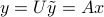 .
.
Example: Assume has the simple form
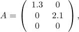
then for an input vector in  , is a vector in
  with first component
  , second component
  , and last component zero.
To summarize, the SVD theorem states that any matrix-vector multiplication can be decomposed as a sequence of three elementary transformations: a rotation in the input space, a scaling that goes from the input space to the output space, and a rotation in the output space. In contrast with symmetric matrices, input and output directions are different.
The interpretation allows to make a few statements about the matrix.
Example: A  example.
Link with the SED
If admits an SVD, then the matrices  and
and  has the following SEDs:

where  is
is  (so it has
  trailing zeros), and
  is
is  (so it has trailing zeros). The eigenvalues of and are the same, and equal to the squared singular values of . The corresponding eigenvectors are the left and right singular vectors of .
This is a method (not the most computationally efficient) to find the SVD of a matrix, based on the SED.