Least-squares and SVD

Set of solutions via the pseudo inverse
Sensitivity analysis
BLUE property

Set of solutions

The following theorem provides all the solutions (optimal set) of a least-squares problem.

Theorem: optimal set of ordinary least-squares

The optimal set of the OLS problem

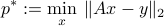
can be expressed as

$mathbf{X}^{rm opt} = A^dagger y + mathbf{N}(A).$

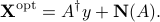
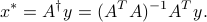
where A^dagger is the pseudo-inverse of , and A^dagger y is the minimum-norm point in the optimal set. If is full column rank, the solution is unique, and equal to

$x^ast = A^dagger y = (A^TA)^{-1} A^Ty.$

In general, the particular solution A^dagger y is the minimum-norm solution to the least-squares problem.

Proof: here.

Sensitivity analysis

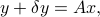
We consider the situation where

with

$A in mathbf{R}^{m times n}$ the data matrix (known), with full column rank (hence ).
$y in mathbf{R}^m$ is the measurement (known).
$x in mathbf{R}^n$ is the vector to be estimated (unknown).
$delta y in mathbf{R}^m$ is a measurement noise or error (unknown).

We can use OLS to provide an estimate $hat{x}_{rm OLS}$ of . The idea is to seek the smallest vector delta y such that the above equation becomes feasible, that is,

$min_{x, delta y} : |delta y|_2 ~:~ y + delta y = Ax .$

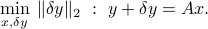
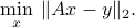
This leads to the OLS problem:

Since is full column rank, its SVD can be expressed as

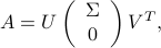
$A = U left( begin{array}{c} Sigma 0 end{array} right) V^T,$

where 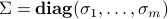$Sigma = mbox{bf diag}(sigma_1,ldots,sigma_m)$ contains the singular values of , with sigma_1 ge ldots ge sigma_m >0 .

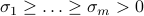Since is full column rank, the solution $hat{x}_{rm LS}$ to the OLS problem is unique, and can be written as a linear function of the measurement vector :

$hat{x}_{rm LS} = A^dagger y,$

with A^dagger the pseudo-inverse of . Again, since is full column rank,

$A^dagger = (A^TA)^{-1}A^T = V left( begin{array}{cc} Sigma^{-1} & 0 end{array} right) U^T.$

The OLS formulation provides an estimate hat{x} of the input such that the residual error vector Ax-y is minimized in norm. We are interested in analyzing the impact of perturbations in the vector , on the resulting solution $hat{x}_{rm LS}$ . We begin by analyzing the absolute errors in the estimate, and then turn to the analysis of relative errors.

Set of possible errors

Let us assume a simple model of potential perturbations: we assume that delta y belongs to a unit ball: |delta y |_2 le alpha , where alpha>0 is given. We will assume alpha = 1 for simplicity; the analysis is easily extended to any alpha >0 .

We have

$begin{array}{rcl} delta x := x-hat{x} &=& x - A^dagger y &=& x - A^dagger (Ax - delta y) &=& (I-A^dagger A) x + A^dagger delta y &=& A^dagger delta y. end{array}$

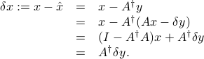
In the above we have exploited the fact that A^dagger is a left inverse of , that is, A^dagger A = I_n .

The set of possible errors on the solution delta x is then given by

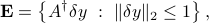
$mathbf{E} = left{ A^dagger delta y ~:~ |delta y|_2 le 1 right},$

which is an ellipsoid centered at zero, with principal axes given by the singular values of A^dagger . This ellipsoid can be interpreted as an ellipsoid of confidence for the estimate hat{x} , with size and shape determined by the matrix A^dagger (A^dagger)^T .

We can draw several conclusions from this analysis:

The largest absolute error in the solution that can result from a unit-norm, additive perturbation on is of the order of , where is the smallest singular value of .
The largest relative error is , the condition number of .

BLUE property

We now return to the case of an OLS with full column rank matrix .

Unbiased linear estimators

Consider the family of linear estimators, which are of the form

where $B in mathbf{R}^{n times m}$ . To this estimator, we associate the error

delta x = x-hat{x} = x - By = x - B(Ax - delta y) = (I-BA) x + B delta y.

We say that the estimator (as determined by matrix ) is unbiased if the first term is zero:

Unbiased estimators only exist when the above equation is feasible, that is, has a left inverse. This is equivalent to our condition that be full column rank. Since A^dagger is a left-inverse of , the OLS estimator is a particular case of an unbiased linear estimator.

Best unbiased linear estimator

The above analysis leads to the following question: which is the best unbiased linear estimator? One way to formulate this problem is to assume that the perturbation vector delta y is bounded in some way, and try to minimize the possible impact of such bounded errors on the solution.

Let us assume that delta y belongs to a unit ball: |delta y |_2 le 1 . The set of resulting errors on the solution delta x is then

$mathbf{E} = left{ B delta y ~:~ |delta|_2 le 1 right},$

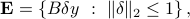
which is an ellipsoid centered at zero, with principal axes given by the singular values of . This ellipsoid can be interpreted as an ellipsoid of confidence for the estimate hat{x} , with size and shape determined by the matrix BB^T .

It can be shown that the OLS estimator is optimal in the sense that it provides the ‘‘smallest’’ ellipsoid of confidence among all unbiased linear estimators. Specifically:

This optimality of the LS estimator is referred to as the BLUE (Best Linear Unbiased Estimator) property.