Definitions
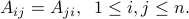
Symmetric matrices and quadratic functions
Second-order approximation of non-linear functions
Special symmetric matrices
Symmetric matrices and quadratic functions
Symmetric matrices
A square matrix  is symmetric if it is equal to its transpose. That is,
The set of symmetric  matrices is denoted
  . This set is a subspace of
  .
.
Examples:
Gram matrix of data points.
 example
Quadratic functions
A function  is said to be a quadratic function if it can be expressed as
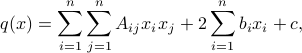
for numbers  ,
,  , and
, and  ,
,  . A quadratic function is thus an affine combination of the
  's and all the ‘‘cross-products’’
  . We observe that the coefficient of is
  .
.
The function is said to be a quadratic form if there are no linear or constant terms in it:  ,
,  .
.
Note that the Hessian (matrix of second-derivatives) of a quadratic function is constant.
Examples:
Link between quadratic functions and symmetric matrices
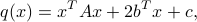
There is a natural relationship between symmetric matrices and quadratic functions. Indeed, any quadratic function can be written as
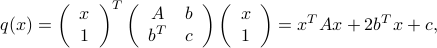
for an appropriate symmetric matrix  , vector
  and scalar
  . Here,
  is the coefficient of
  in
in  ; for
; for  ,
,  is the coefficient of the term in ;
  is that of ; and is the constant term,
  . If is a quadratic form, then
  , , and we can write
  where now
  .
.
Examples:
Second-order approximations of non-quadratic functions
We have seen here how linear functions arise when one seeks a simple, linear approximation to a more complicated non-linear function. Likewise, quadratic functions arise naturally when one seeks to approximate a given non-quadratic function by a quadratic one.
One-dimensional case
If  is a twice-differentiable function of a single variable, then the second order approximation (or, second-order Taylor expansion) of
  at a point
  is of the form

where  is the first derivative, and
  the second derivative, of at . We observe that the quadratic approximation has the same value, derivative, and second-derivative as , at .
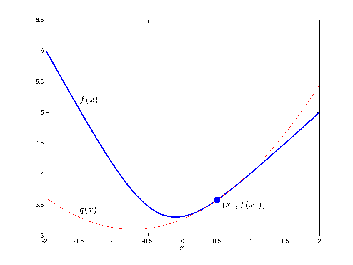 |
Example: The figure shows a second-order approximation 
at the point |
 (in red).
 Multi-dimensional case
In multiple dimensions, we have a similar result. Let us approximate a twice-differentiable function  by a quadratic function , so that and coincide up and including to the second derivatives.
The function must be of the form
where , , and  . Our condition that coincides with up and including to the second derivatives shows that we must have

where  is the Hessian, and
  the gradient, of at .
Solving for  we obtain the following result:
Second-order expansion of a function.
The second-order approximation ofa twice-differentiable function at a point is of the form

where  is the gradient of at , and the symmetric matrix is the Hessian of at .
Example: Second-order expansion of the log-sum-exp function.
Special symmetric matrices
Diagonal matrices
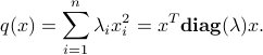
Perhaps the simplest special case of symmetric matrices is the class of diagonal matrices, which are non-zero only on their diagonal.
If  , we denote by
  , or
, or  for short, the (symmetric) diagonal matrix with
  on its diagonal. Diagonal matrices correspond to quadratic functions of the form
Such functions do not have any ‘‘cross-terms’’ of the form  with .
Example: A diagonal matrix and its associated quadratic form.
Symmetric dyads
Another important class of symmetric matrices is that of the form  , where
  . The matrix has elements
  , and is symmetric. Such matrices are called symmetric dyads. (If
  , then the dyad is said to be normalized.)
Symmetric dyads corresponds to quadratic functions that are simply squared linear forms: 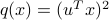 .
.
Example: A squared linear form.