4.3 Value Iteration
Now that we have a framework to test for the optimality of the values of states in an MDP, the natural follow-up question is how to actually compute these optimal values. To answer this, we need time-limited values (the natural result of enforcing finite horizons). The time-limited value for a state \(s\) with a time limit of \(k\) timesteps is denoted \(V_k(s)\), and represents the maximum expected utility attainable from \(s\) given that the Markov decision process under consideration terminates in \(k\) timesteps. Equivalently, this is what a depth-\(k\) expectimax run on the search tree for an MDP returns.
Value iteration is a dynamic programming algorithm that uses an iteratively longer time limit to compute time-limited values until convergence (that is, until the \(V\) values are the same for each state as they were in the past iteration: \(\forall s, V_{k+1}(s) = V_{k}(s)\)). It operates as follows:
- \(\forall s \in S,\) initialize \(V_0(s) = 0\). This should be intuitive, since setting a time limit of 0 timesteps means no actions can be taken before termination, and so no rewards can be acquired.
-
Repeat the following update rule until convergence:
\[\forall s \in S, \:\: V_{k+1}(s) \leftarrow \max_a \sum_{s'}T(s, a, s')[R(s, a, s') + \gamma V_k(s')]\]At iteration \(k\) of value iteration, we use the time-limited values with limit \(k\) for each state to generate the time-limited values with limit \((k+1)\). In essence, we use computed solutions to subproblems (all the \(V_k(s)\)) to iteratively build up solutions to larger subproblems (all the \(V_{k+1}(s)\)); this is what makes value iteration a dynamic programming algorithm.
Note that though the Bellman equation looks essentially identical to the update rule above, they are not the same. The Bellman equation gives a condition for optimality, while the update rule gives a method to iteratively update values until convergence. When convergence is reached, the Bellman equation will hold for every state: \(\forall s \in S, \:\: V_k(s) = V_{k+1}(s) = V^*(s)\).
For conciseness, we frequently denote \(U_{k+1}(s) \leftarrow \max_a \sum_{s'}T(s, a, s')[R(s, a, s') + \gamma V_k(s')]\) with the shorthand \(V_{k+1} \leftarrow BU_k\), where \(B\) is called the Bellman operator. The Bellman operator is a contraction by \(\gamma\). To prove this, we will need the following general inequality:
\[| \max_z f(z) - \max_z h(z) | \leq \max_z |f(z) - h(z)|.\]Now consider two value functions evaluated at the same state \(V(s)\) and \(V'(s)\). We show that the Bellman update \(B\) is a contraction by \(\gamma \in (0, 1)\) with respect to the max norm as follows:
\(\begin{aligned} &|BV(s) - BV'(s)| \\ &= \left| \left( \max_a \sum_{s'}T(s, a, s')[R(s, a, s') + \gamma V(s')] \right) - \left( \max_a \sum_{s'}T(s, a, s')[R(s, a, s') + \gamma V'(s')] \right) \right| \\ &\leq \max_a \left| \sum_{s'}T(s, a, s')[R(s, a, s') + \gamma V(s')] - \sum_{s'}T(s, a, s')[R(s, a, s') + \gamma V'(s')] \right| \\ &= \max_a \left| \gamma \sum_{s'}T(s, a, s')V(s') - \gamma \sum_{s'}T(s, a, s')V'(s') \right| \\ &= \gamma \max_a \left| \sum_{s'}T(s, a, s')(V(s') - V'(s')) \right| \\ &\leq \gamma \max_a \left| \sum_{s'}T(s, a, s') \max_{s'} \left| V(s') - V'(s') \right| \right| \\ &= \gamma \max_{s'} \left| V(s') - V'(s') \right| \\ &= \gamma ||V(s') - V'(s')||_{\infty}, \end{aligned}\)
where the first inequality follows from the general inequality introduced above, the second inequality follows from taking the maximum of the differences between \(V\) and \(V'\), and in the second-to-last step, we use the fact that probabilities sum to 1 no matter the choice of \(a\). The last step uses the definition of the max norm for a vector \(x = (x_1, \ldots, x_n)\), which is \(||x||_{\infty} = \max(|x_1|, \ldots, |x_n|)\).
Because we just proved that value iteration via Bellman updates is a contraction in \(\gamma\), we know that value iteration converges, and convergence happens when we have reached a fixed point that satisfies \(V^* = BU^*\).
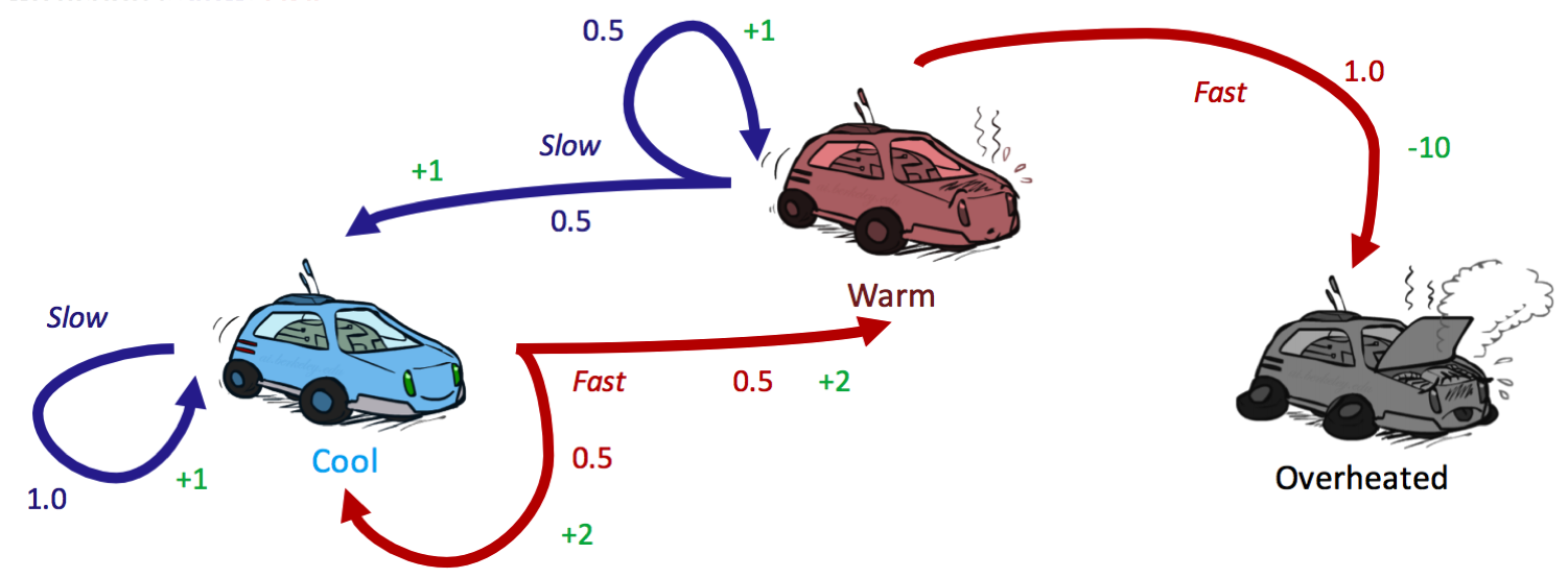
Let’s see a few updates of value iteration in practice by revisiting our racecar MDP from earlier, introducing a discount factor of \(\gamma = 0.5\):
We begin value iteration by initializing all \(V_0(s) = 0\):
| cool | warm | overheated | |
|---|---|---|---|
| \(V_0\) | 0 | 0 | 0 |
In our first round of updates, we can compute \(\forall s \in S, \:\: V_1(s)\) as follows:
\[\begin{aligned} V_1(cool) &= \max \{1 \cdot [1 + 0.5 \cdot 0],\:\: 0.5 \cdot [2 + 0.5 \cdot 0] + 0.5 \cdot [2 + 0.5 \cdot 0]\} \\ &= \max \{1, 2\} \\ &= \boxed{2} \\ V_1(warm) &= \max \{0.5 \cdot [1 + 0.5 \cdot 0] + 0.5 \cdot [1 + 0.5 \cdot 0],\:\: 1 \cdot [-10 + 0.5 \cdot 0]\} \\ &= \max \{1, -10\} \\ &= \boxed{1} \\ V_1(overheated) &= \max \{\} \\ &= \boxed{0} \end{aligned}\]| cool | warm | overheated | |
|---|---|---|---|
| \(U_0\) | 0 | 0 | 0 |
| \(U_1\) | 2 | 1 | 0 |
Similarly, we can repeat the procedure to compute a second round of updates with our newfound values for \(U_1(s)\) to compute \(V_2(s)\):
\[\begin{aligned} V_2(cool) &= \max \{1 \cdot [1 + 0.5 \cdot 2],\:\: 0.5 \cdot [2 + 0.5 \cdot 2] + 0.5 \cdot [2 + 0.5 \cdot 1]\} \\ &= \max \{2, 2.75\} \\ &= \boxed{2.75} \\ V_2(warm) &= \max \{0.5 \cdot [1 + 0.5 \cdot 2] + 0.5 \cdot [1 + 0.5 \cdot 1],\:\: 1 \cdot [-10 + 0.5 \cdot 0]\} \\ &= \max \{1.75, -10\} \\ &= \boxed{1.75} \\ V_2(overheated) &= \max \{\} \\ &= \boxed{0} \end{aligned}\]| cool | warm | overheated | |
|---|---|---|---|
| \(V_0\) | 0 | 0 | 0 |
| \(V_1\) | 2 | 1 | 0 |
| \(V_2\) | 2.75 | 1.75 | 0 |
It’s worthwhile to observe that \(V^*(s)\) for any terminal state must be 0, since no actions can ever be taken from any terminal state to reap any rewards.
4.3.1 Policy Extraction
Recall that our ultimate goal in solving an MDP is to determine an optimal policy. This can be done once all optimal values for states are determined using a method called policy extraction. The intuition behind policy extraction is very simple: if you’re in a state \(s\), you should take the action \(a\) which yields the maximum expected utility. Not surprisingly, \(a\) is the action which takes us to the Q-state with maximum Q-value, allowing for a formal definition of the optimal policy:
\[\forall s \in S, \:\: \pi^*(s) = \underset{a}{\operatorname{argmax}}\: Q^*(s, a) = \underset{a}{\operatorname{argmax}}\: \sum_{s'}T(s, a, s')[R(s, a, s') + \gamma V^*(s')]\]It’s useful to keep in mind for performance reasons that it’s better for policy extraction to have the optimal Q-values of states, in which case a single \(\operatorname{argmax}\) operation is all that is required to determine the optimal action from a state. Storing only each \(V^*(s)\) means that we must recompute all necessary Q-values with the Bellman equation before applying \(\operatorname{argmax}\), equivalent to performing a depth-1 expectimax.
4.3.2 Q-Value Iteration
In solving for an optimal policy using value iteration, we first find all the optimal values, then extract the policy using policy extraction. However, you might have noticed that we also deal with another type of value that encodes information about the optimal policy: Q-values.
Q-value iteration is a dynamic programming algorithm that computes time-limited Q-values. It is described in the following equation:
\[Q_{k+1}(s, a) \leftarrow \sum_{s'}T(s, a, s')[R(s, a, s') + \gamma \max_{a'} Q_k(s', a')]\]Note that this update is only a slight modification over the update rule for value iteration. Indeed, the only real difference is that the position of the \(\max\) operator over actions has been changed since we select an action before transitioning when we’re in a state, but we transition before selecting a new action when we’re in a Q-state. Once we have the optimal Q-values for each state and action, we can then find the policy for a state by simply choosing the action which has the highest Q-value.