7.2 Decision Networks

Previously we learned about game trees and algorithms such as minimax and expectimax, which we used to determine optimal actions that maximized our expected utility. Then in the fifth note, we discussed Bayes’ nets and how we can use evidence we know to run probabilistic inference to make predictions. Now we’ll discuss a combination of both Bayes’ nets and expectimax known as a decision network that we can use to model the effect of various actions on utilities based on an overarching graphical probabilistic model. Let’s dive right in with the anatomy of a decision network:

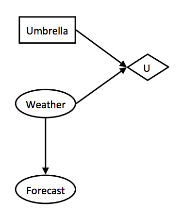
• Chance nodes - Chance nodes in a decision network behave identically to Bayes’ nets. Each outcome in a chance node has an associated probability, which can be determined by running inference on the underlying Bayes’ net it belongs to. We’ll represent these with ovals.
• Action nodes - Action nodes are nodes that we have complete control over; they’re nodes representing a choice between any of a number of actions which we have the power to choose from. We’ll represent action nodes with rectangles.
• Utility nodes - Utility nodes are children of some combination of action and chance nodes. They output a utility based on the values taken on by their parents, and are represented as diamonds in our decision networks.

Consider a situation when you’re deciding whether or not to take an umbrella when you’re leaving for class in the morning, and you know there’s a forecasted 30% chance of rain. Should you take the umbrella? If there was an 80% chance of rain, would your answer change? This situation is ideal for modeling with a decision network, and we do it as follows:

As we’ve done throughout this course with the various modeling techniques and algorithms we’ve discussed, our goal with decision networks is again to select the action which yields the maximum expected utility (MEU). This can be done with a fairly straightforward and intuitive procedure:

• Start by instantiating all evidence that’s known, and run inference to calculate the posterior probabilities of all chance node parents of the utility node into which the action node feeds.

• Go through each possible action and compute the expected utility of taking that action given the posterior probabilities computed in the previous step. The expected utility of taking an action \(a\) given evidence \(e\) and \(n\) chance nodes is computed with the following formula:

  \[EU(a \mid e) = \sum_{x_1, ..., x_n}P(x_1, ..., x_n \mid e)U(a, x_1, ..., x_n)\]

  where each \(x_i\) represents a value that the \(i^{th}\) chance node can take on. We simply take a weighted sum over the utilities of each outcome under our given action with weights corresponding to the probabilities of each outcome.

• Finally, select the action which yielded the highest utility to get the MEU.

Let’s see how this actually looks by calculating the optimal action (should we leave or take our umbrella) for our weather example, using both the conditional probability table for weather given a bad weather forecast (forecast is our evidence variable) and the utility table given our action and the weather:

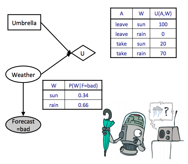
Note that we have omitted the inference computation for the posterior probabilities $P(W \mid F = \text{bad})$, but we could compute these using any of the inference algorithms we discussed for Bayes Nets. Instead, here we simply assume the above table of posterior probabilities for $P(W \mid F = \text{bad})$ as given. Going through both our actions and computing expected utilities yields:

\[\begin{aligned} EU(\text{leave} \mid \text{bad}) &= \sum_{w}P(w \mid \text{bad})U(\text{leave}, w) \\ &= 0.34 \cdot 100 + 0.66 \cdot 0 = \boxed{34} \\ EU(\text{take} \mid \text{bad}) &= \sum_{w}P(w \mid \text{bad})U(\text{take}, w) \\ &= 0.34 \cdot 20 + 0.66 \cdot 70 = \boxed{53} \end{aligned}\]

All that’s left to do is take the maximum over these computed utilities to determine the MEU:

\[MEU(F = \text{bad}) = \max_aEU(a \mid \text{bad}) = \boxed{53}\]

The action that yields the maximum expected utility is take, and so this is the action recommended to us by the decision network. More formally, the action that yields the MEU can be determined by taking the argmax over expected utilities.

7.2.1 Outcome Trees

We mentioned at the start of this note that decision networks involved some expectimax-esque elements, so let’s discuss what exactly that means. We can unravel the selection of an action corresponding to the one that maximizes expected utility in a decision network as an outcome tree. Our weather forecast example from above unravels into the following outcome tree:

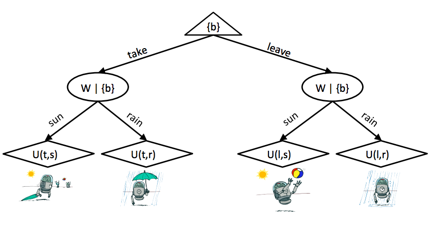
The root node at the top is a maximizer node, just like in expectimax, and is controlled by us. We select an action, which takes us to the next level in the tree, controlled by chance nodes. At this level, chance nodes resolve to different utility nodes at the final level with probabilities corresponding to the posterior probabilities derived from probabilistic inference run on the underlying Bayes’ net. What exactly makes this different from vanilla expectimax? The only real difference is that for outcome trees we annotate our nodes with what we know at any given moment (inside the curly braces).