7.3 The Value of Perfect Information
In everything we’ve covered up to this point, we’ve generally always assumed that our agent has all the information it needs for a particular problem and/or has no way to acquire new information. In practice, this is hardly the case, and one of the most important parts of decision making is knowing whether or not it’s worth gathering more evidence to help decide which action to take. Observing new evidence almost always has some cost, whether it be in terms of time, money, or some other medium. In this section, we’ll talk about a very important concept - the value of perfect information (VPI) - which mathematically quantifies the amount an agent’s maximum expected utility is expected to increase if it observes some new evidence. We can compare the VPI of learning some new information with the cost associated with observing that information to make decisions about whether or not it’s worthwhile to observe.
7.3.1 General Formula
Rather than simply presenting the formula for computing the value of perfect information for new evidence, let’s walk through an intuitive derivation. We know from our above definition that the value of perfect information is the amount our maximum expected utility is expected to increase if we decide to observe new evidence. We know our current maximum utility given our current evidence \(e\):
\[MEU(e) = \max_a\sum_sP(s \mid e)U(s, a)\]Additionally, we know that if we observed some new evidence \(e'\) before acting, the maximum expected utility of our action at that point would become
\[MEU(e, e') = \max_a\sum_sP(s \mid e, e')U(s, a)\]However, note that we don’t know what new evidence we’ll get. For example, if we didn’t know the weather forecast beforehand and chose to observe it, the forecast we observe might be either good or bad. Because we don’t know what new evidence \(e'\) we’ll get, we must represent it as a random variable \(E'\). How do we represent the new MEU we’ll get if we choose to observe a new variable if we don’t know what the evidence gained from observation will tell us? The answer is to compute the expected value of the maximum expected utility which, while being a mouthful, is the natural way to go:
\[MEU(e, E') = \sum_{e'}P(e' \mid e)MEU(e, e')\]Observing a new evidence variable yields a different MEU with probabilities corresponding to the probabilities of observing each value for the evidence variable, and so by computing \(MEU(e, E')\) as above, we compute what we expect our new MEU will be if we choose to observe new evidence. We’re just about done now - returning to our definition for VPI, we want to find the amount our MEU is expected to increase if we choose to observe new evidence. We know our current MEU and the expected value of the new MEU if we choose to observe, so the expected MEU increase is simply the difference of these two terms! Indeed,
\[\boxed{VPI(E' \mid e) = MEU(e, E') - MEU(e)}\]where we can read \(VPI(E' \mid e)\) as “the value of observing new evidence E’ given our current evidence e”. Let’s work our way through an example by revisiting our weather scenario one last time:
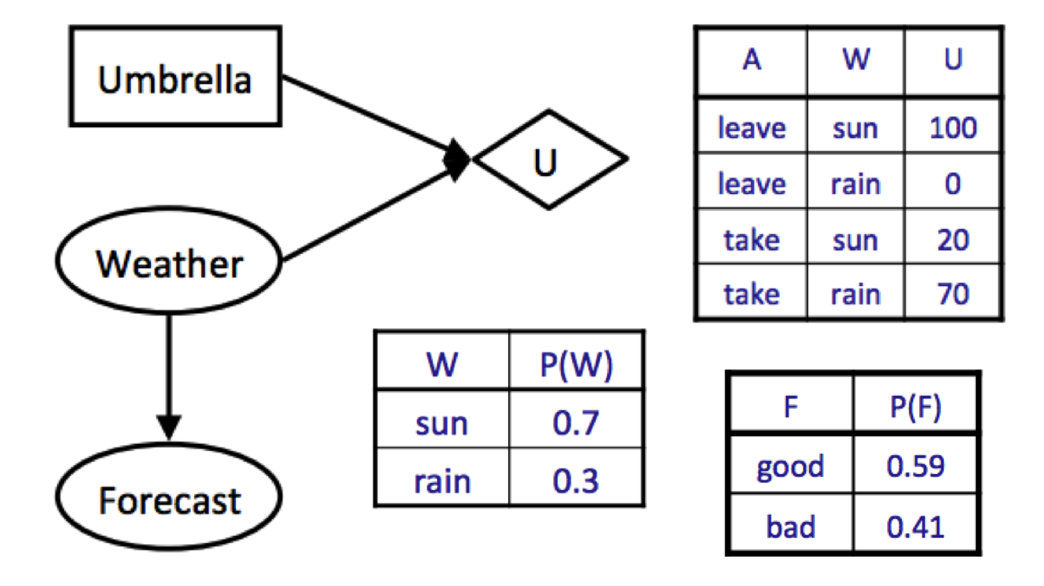
If we don’t observe any evidence, then our maximum expected utility can be computed as follows:
\[\begin{aligned} MEU(\varnothing) &= \max_aEU(a) \\ &= \max_a\sum_wP(w)U(a, w) \\ &= \max\{0.7 \cdot 100 + 0.3 \cdot 0, 0.7 \cdot 20 + 0.3 \cdot 70\} \\ &= \max\{70, 35\} \\ &= 70 \end{aligned}\]Note that the convention when we have no evidence is to write \(MEU(\varnothing)\), denoting that our evidence is the empty set. Now let’s say that we’re deciding whether or not to observe the weather forecast. We’ve already computed that \(MEU(F = \text{bad}) = 53\), and let’s assume that running an identical computation for \(F = \text{good}\) yields \(MEU(F = \text{good}) = 95\). We’re now ready to compute \(MEU(e, E')\):
\[\begin{aligned} MEU(e, E') &= MEU(F) \\ &= \sum_{e'}P(e' \mid e)MEU(e, e') \\ &= \sum_{f}P(F = f)MEU(F = f) \\ &= P(F = \text{good})MEU(F = \text{good}) + P(F = \text{bad})MEU(F = \text{bad}) \\ &= 0.59 \cdot 95 + 0.41 \cdot 53 \\ &= 77.78 \end{aligned}\]Hence we conclude \(VPI(F) = MEU(F) - MEU(\varnothing) = 77.78 - 70 = \boxed{7.78}\).
7.3.2 Properties of VPI
The value of perfect information has several very important properties, namely:
-
Nonnegativity. \(\forall E', e\:\: VPI(E' \mid e) \geq 0\)
Observing new information always allows you to make a more informed decision, and so your maximum expected utility can only increase (or stay the same if the information is irrelevant for the decision you must make). -
Nonadditivity. \(VPI(E_j, E_k \mid e) \neq VPI(E_j \mid e) + VPI(E_k \mid e)\) in general.
This is probably the trickiest of the three properties to understand intuitively. It’s true because generally observing some new evidence \(E_j\) might change how much we care about \(E_k\); therefore we can’t simply add the VPI of observing \(E_j\) to the VPI of observing \(E_k\) to get the VPI of observing both of them. Rather, the VPI of observing two new evidence variables is equivalent to observing one, incorporating it into our current evidence, then observing the other. This is encapsulated by the order-independence property of VPI, described more below. -
Order-independence. \(VPI(E_j, E_k \mid e) = VPI(E_j \mid e) + VPI(E_k \mid e, E_j) = VPI(E_k \mid e) + VPI(E_j \mid e, E_k)\)
Observing multiple new evidences yields the same gain in maximum expected utility regardless of the order of observation. This should be a fairly straightforward assumption - because we don’t actually take any action until after observing any new evidence variables, it doesn’t actually matter whether we observe the new evidence variables together or in some arbitrary sequential order.