Linear Matrix Inequalities
Definition
LMIs and convex sets
Special cases
Definition
Positive Semi-Definite Matrices
Recall from here that a  symmetric matrix
  is positive semi-definite (PSD) if and only if every one of its eigenvalues is non-negative. We use the notation
  to mean that is PSD.
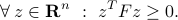
An alternative condition for to be PSD is that the associated quadratic form is non-negative:
The set of PSD matrices is convex, since the conditions above represent (an infinite number of) ordinary linear inequalities on the elements of the matrix .
Examples:
For any vector
 , the dyad
  is PSD, since the associated quadratic form is
  .
.More generally, for any rectangular matrix
 , the ‘‘square’’ matrix
  is PSD.
The converse is true: any PSD matrix can be factored as
 for some appropriate matrix .
 example
Standard form
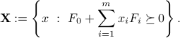
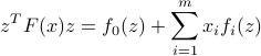
A linear matrix inequality is a constraint of the form
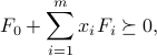
where the matrices  are symmetric.
 |
An LMI in two variables: 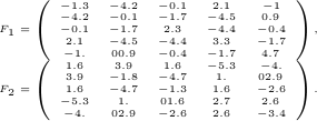
|
 , where
  are the two
  symmetric matrices
The matrices are referred to as the coefficient matrices. Sometimes, these matrices are not explicitly defined. That is, if  is an affine map that takes its values in the set of symmetric matrices of order
  , then
  is an LMI.
An alternate form for LMIs is as the intersection of the positive semi-definite cone with an affine set:
where  is affine. The form we have seen before, and the above one, are equivalent, in the sense that we can always transform one into the other (at the expense possibly of adding new variables and constraints).
LMIs and Convex Sets
Let us denote by  the set of points
  that satisfy the above LMI.
The set is convex. Indeed, we have if and only if
Since
with  ,
,  , we obtain that the condition on
  :
:  can be represented as an intersection of (an infinite number of) half-space conditions.
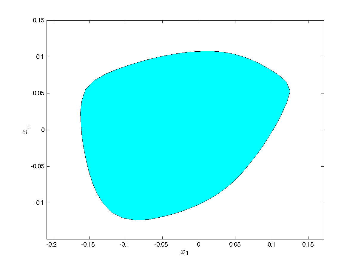
 |
Supporting hyperplanes: The picture shows how the set seen above can be interpreted as the intersection of a number of half-spaces. Each half-space corresponds to an affine inequality of the form |
 , for a specific vector
  . The vectors
 Multiple LMIs
We can combine multiple LMIs into one. Consider two affine maps from  to a space of symmetric matrices of order
  ,
,  ,
,  . Then the two LMIs
are equivalent to one LMI, involving a larger matrix of size  :
:
This corresponds to intersecting the two LMI sets.
Special Cases
LMIs include as special cases the following.
Ordinary affine inequalities
Consider single affine inequality in  :
:

where  ,
,  . (The above set describes a half-space.) The above is a trivial special case of LMI, where the coefficient matrices are scalar:
  ,
,  ,
,  .
.
Using the result above on multiple LMIs, we obtain that the set of ordinary affine inequalities
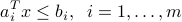
can be cast as a single LMI , where
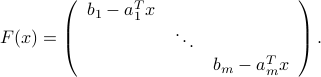
Second-order cone inequalities
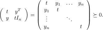
Second-order cone (SOC) inequalities can be represented as LMIs. To see this, let us start with the ‘‘basic’’ SOC  , with
  and
and  . The SOC can be represented as
Indeed, we check that for every  ,
,  , we have

if and only if .
More generally, a second-order cone inequality of the form
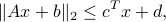
with  ,
,  ,
,  ,
,  , can be written as the LMI
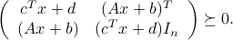
The proof relies on the Schur complement lemma.