Algorithms for Convex Optimization

Convex Optimization > Convex sets | Convex functions | Convex optimization problems | Algorithms | DCP

From Least-Squares to convex minimization
Unconstrained minimization via Newton's method
Interior-point methods
Gradient methods

From Least-Squares to convex minimization

We have seen how ordinary least-squares (OLS) problems can be solved using linear algebra (e.g. SVD) methods. Using OLS, we can minimize convex, quadratic functions of the form

$q(x) = frac{1}{2} x^THx + g^Tx$

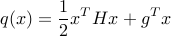
when 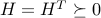H=H^T succeq 0 . This last requirement ensures that the function is convex. For such convex quadratic functions, as for any convex functions, any local minimum is global. In fact, when H succ 0 , then the unique minimizer is $x^star = - H^{-1}g$ .

It turns out one can leverage the approach to minimizing more general functions, using an iterative algorithm, based on a local quadratic approximation of the the function at the current point. The approach can then be extended to problems with constraints, by replacing the original constrained problem with an unconstrained one, in which the constraints are penalized in the objective.

Unconstrained minimization: Newton's method

We consider an unconstrained minimization problem, where we seek to minimize a function twice-differentiable function . Let us assume that the function under consideration is strictly convex, which is to say that its Hessian is positive definite everywhere. (If is not convex, we might run into a local minima.)

For minimizing convex functions, an iterative procedure could be based on a simple quadratic approximation procedure known as Newton's method. We start with initial guess x_0 . At each step , we update our current guess x_t by minimizing the second-order approximation tilde{f} of at x_t , which is the quadratic function (see here)

$tilde{f}(x) := f(x_t) + nabla f(x_t)^T(x-x_t) + frac{1}{2} (x-x_t)^T nabla^2 f(x_t) (x-x_t),$

where nabla f(x_t) denotes the gradient, and nabla^2 f(x_t) the Hessian, of at x_t . Our next guess $x_{t+1}$ , will be set to be a solution to the problem of minimizing tilde{f} . Since the function is strictly convex, we have nabla^2 f(x_0) succ 0 , so that the problem we are solving at each step has a unique solution, which corresponds to the global minimum of . The basic Newton iteration is thus

$x_{t+1} = x_t - (nabla^2 f(x_t))^{-1} nabla f(x_t)$

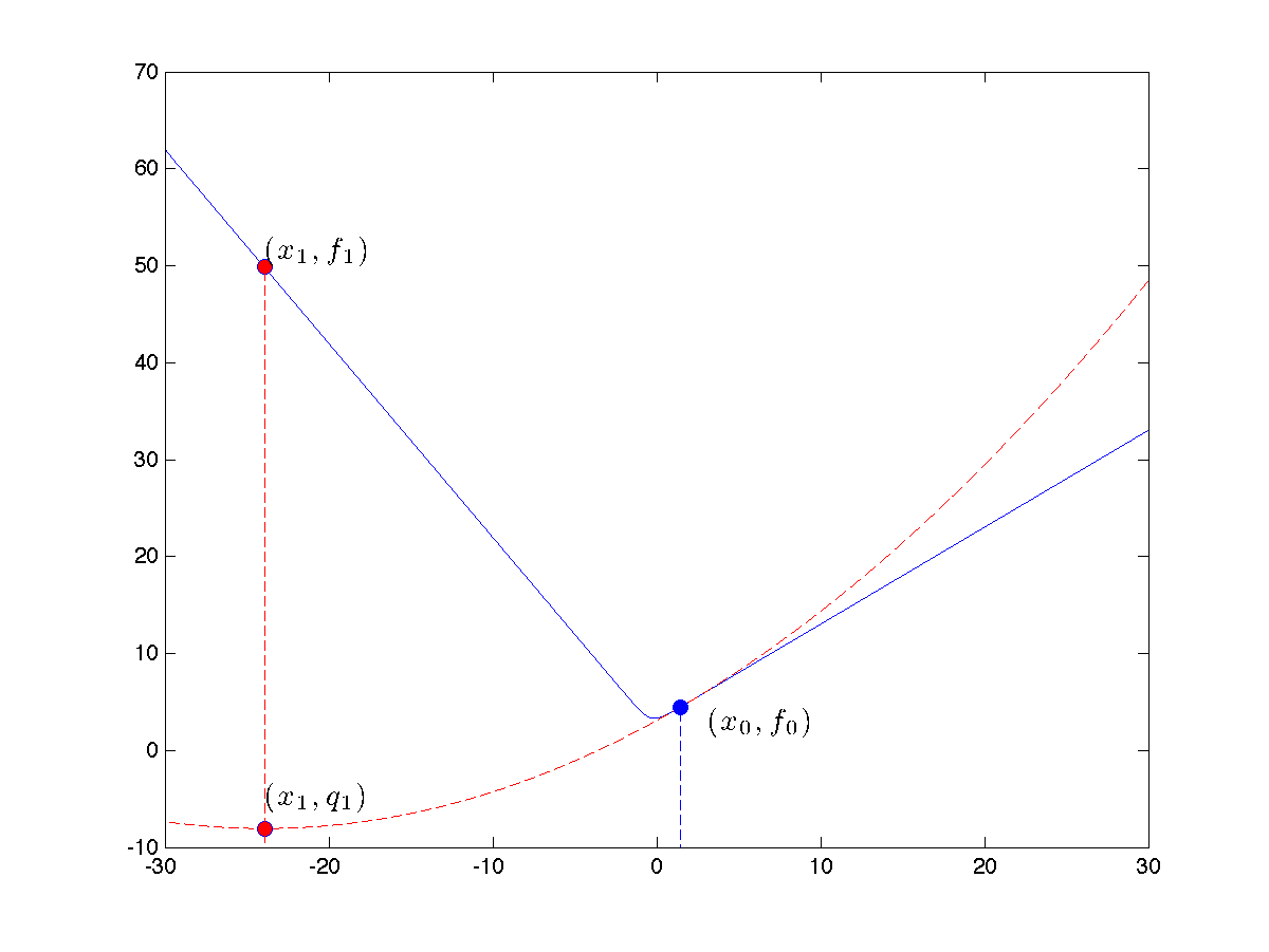
Two initial steps of Newton's method to minimize the function $f : mathbf{R}^2 rightarrow mathbf{R}$ with domain the whole $mathbf{R}^2$ , and values

A first local quadratic approximation at the initial point x_0 = 0.5 is formed (dotted line in green). The corresponding minimizer is the new iterate, x_1 . The Newton algorithm proceeds to form a new quadratic approximation of the function at that point (dotted line in red), leading to the second iterate, x_2 . Although x_1 turns out to be further away from the global minimizer x^ast (in light blue), x_2 is closer, and the method actually converges quickly.

This idea will fail for general (non-convex) functions. It might even fail for some convex functions. However, for a large class of convex functions, knwon as self-concordant functions, a variation on the Newton method works extremely well, and is guaranteed to find the global minimizer of the function . For such functions, the Hessian does not vary too fast, which turns out to be a crucial ingredient for the success of Newton's method.

Failure of the Newton method to minimize the above convex function. The initial point is chosen too far away from the global minimizer x^ast , in a region where the function is almost linear. As a result, the quadratic approximation is almost a straight line, and the Hessian is close to zero, sending the first iterate of Newton's method to a relatively large negative value. The method quickly diverges in this case, with a second iterate at $x_2 approx 2 e^{30}$ .

Constrained minimization: interior-point methods

The method above can be applied to the more general context of convex optimization problems of standard form:

$displaystylemin_x : f_0(x) mbox{ subject to } f_i(x) le 0, ;; i=1,ldots, m ,$

where every function involved is twice-differentiable, and convex.

The basic idea behind interior-point methods is to replace the constrained problem by an unconstrained one, involving a function that is constructed with the original problem functions. One further idea is to use a logarithmic barrier: in lieu of the original problem, we address

$min_x : f(x) := f_0(x) - mu sum_{i=1}^m log ( -f_i(x) ),$

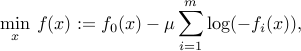
where mu>0 is a small parameter. The function turns out to be convex, as long as f_0,ldots,f_m are.

For large, solving the above problem results in a point well ‘‘inside’’ the feasible set, an ‘‘interior point’’. As mu rightarrow 0 the solution converges to a global minimizer for the original, constrained problem. In fact, the theory of convex optimization says that if we set mu = m/epsilon , then a minimizer to the above function is epsilon -suboptimal. In practice, algorithms do not set the value of so aggressively, and update the value of a few times.

For a large class of convex optimization problems, the function is self-concordant, so that we can safely apply Newton's method to the minimization of the above function. In fact, for a large class of convex optimization problems, the method converges in time polynomial in .

The interior-point approach is limited by the need to form the gradient and Hessian of the function above. For extremely large-scale problems, this task may be too daunting.

Gradient methods

Unconstrained case

Gradient methods offer an alternative to interior-point methods, which is attractive for large-scale problems. Typically, these algorithms need a considerably larger number of iterations compared to interior-point methods, but each iteration is much cheaper to process.

Perhaps the simplest algorithm to minimizing a convex function involves the iteration

$x_{t+1} = x_t - alpha_t nabla f(x_t) ,$

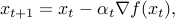
where alpha_t>0 is a parameter. The interpretation of the algorithm is that it tries to decrease the value of the function by taking a step in the direction of the negative gradient. For small enough value of alpha_t , indeed we have $f(x_{t+1}) le f(x_t)$ .

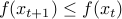Depending on the choice of the parameter alpha_t (as as function of the iteration number ), and some properties on the function , convergence can be rigorously proven.

Constrained case

The gradient method can be adapted to constrained problems, via the iteration

$x_{t+1} = P(x_t - alpha_t nabla f(x)_t),$

where is the projection operator, which to its argument associates the point closest (in Euclidean norm sense) to in mathbf{C} . Depending on problem structure, this projection may or may not be easy to perform.

Example: Box-constrained least-squares.